What happens behind the scenes when you interact with a Grasshopper model on ShapeDiver? What's the difference versus doing the same on your desktop? We've heard these questions numerous times, so finally, we're sharing the full scope.

When working with parametric models, many users expect the same swift interaction from ShapeDiver as they experience in Rhino on their desktops. While this is completely understandable, there are many additional steps between the initial parameter change and the final delivery of the solution to your browser.

Below we go into detail about each of these steps, and we provide some insight into our strategies to improve the response times of your ShapeDiver models.

Computation Time & Response Time

With Grasshopper, the main factor determining how fast models are updated is the computation time of a definition. In other words, how much time it takes for Rhino to solve the definition for a specific set of inputs? On top of the computation time, Rhino also takes some time to render the geometry in the viewport, but this is usually a fraction of the computation time.

Computation time is a key value in the ShapeDiver context for two reasons:

1. Our pricing model is based on it: Free accounts get 10 seconds, Designer and Designer Plus accounts 10 or option for 30 seconds, and Business gets 30 or option for 60 seconds. Enterprise accounts get unlimited time.

2. It impacts the performance of your models and therefore plays a strong role in making or breaking the user experience of the ShapeDiver model.

However, computation time is only a subset of the total response time that users experience when changing parameters and interacting with a ShapeDiver model.

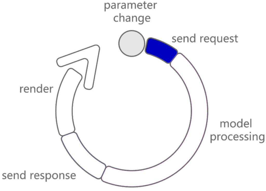
The response time represents the total time elapsed between a request from the ShapeDiver model (for example, the end users updating a parameter) and the moment when the solution is received and displayed in the web browser. Overall, this time is the important one to consider for a smooth and enjoyable user experience. From the moment a user tweaks a slider, a number of things happen until the viewer refreshes so let’s break down those steps.

Step 1: Send Request

Immediately after a parameter change, a JSON object with the new parameter values is sent from the web browser to our servers. The object itself is quite tiny in size and should hit our servers in a fraction of a second. Bear in mind fluctuations might happen as this depends entirely on the Internet speed and network status of each user, factors that, sadly, we can’t influence yet.

Developers can find out more about the API calls that are triggered when changing a parameter in our documentation section.

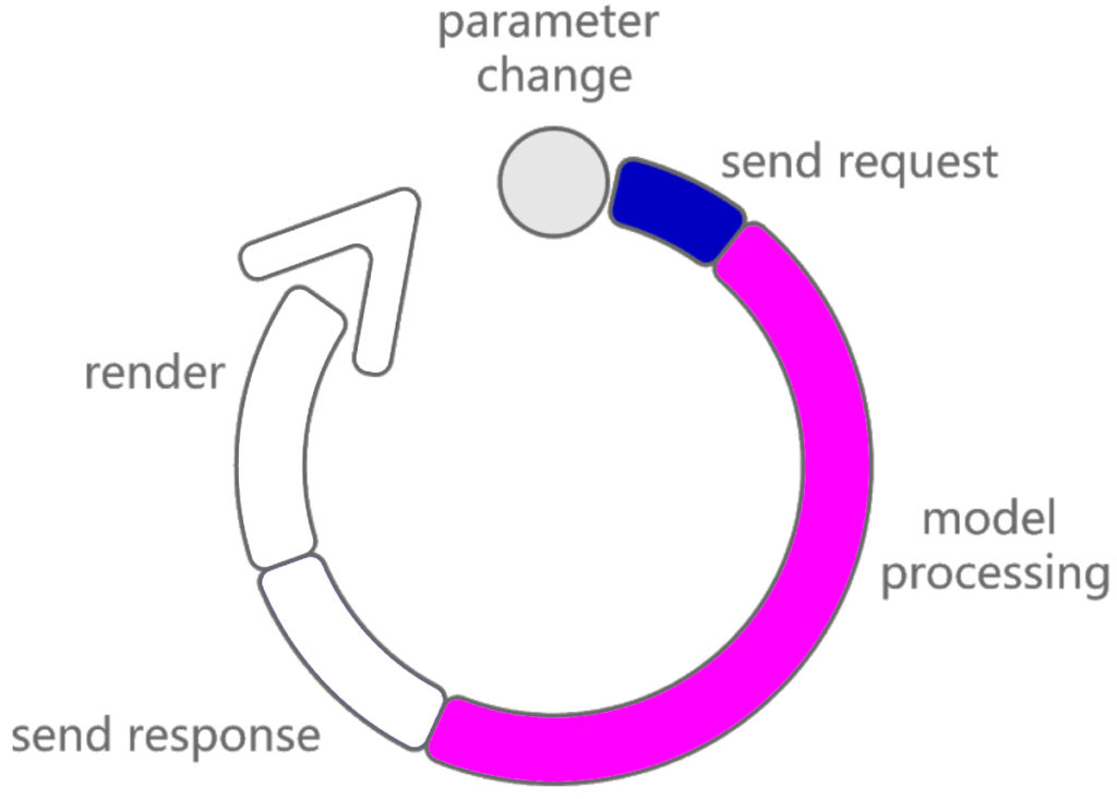
Step 2: Model Processing (Computation Time)

After the parameter update request has successfully arrived, the processing of the model starts. In this step, our servers actually run the Grasshopper definition and compute a solution from it. In other words, we are talking about the computation time of the Grasshopper file stored in our system. 

It’s hard to predict computation times, but as a rule of thumb, we can assume that the processing on our shared system is about the same as you’d expect on your laptop.

Regarding this step, Grasshopper experts can make a huge difference and cut down the overall response time by making their parametric models as efficient as possible. Therefore optimize, optimize, optimize!

* Learn more about different optimization methods in our video tutorials.

Bonus Step: Caching System + CDN

In order to reduce the processing time even further, we developed a system that combines caching assets with Content Delivery Networks to achieve blazing-fast geometry delivery.

Basically, we store all previously computed states for any given model. This means that if a user chooses a parameter combination that our system has previously processed, our system no longer has to use the Grasshopper file to generate the result. Instead, a cached solution is fetched and sent.

In the model above, both the Spokes (11 variations) and Subdivisions (19 variations) parameters are fully cached in our system. For any combination of these two parameters (209 in total), results are sent from our caching system and not from the Grasshopper file. All the other parameters are not fully cached, so the configurator has to wait for the answer to be computed from scratch.

You can use this to your advantage if your configurator has a manageable amount of parameters that you or someone from your team could "warm up" ahead of time.

* Learn more about the smart caching in this article.

Step 3: Send Response

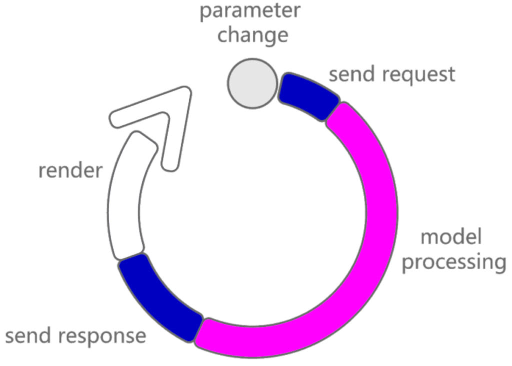
Once a solution is computed, it is stored in a cloud-optimized geometry format (gltf) and travels back to the user’s web browser. The same network factors come into play as with Step 1, though this step can take up to a few seconds as the server sends meshes instead of a simple JSON object. This means that the size of the output geometry plays a significant role in response time. These are large chunks of data, so keep the output limits in mind when working on the Grasshopper definition.

Various optimization and meshing techniques are well covered in this article, video tutorial and the webinar. 

Step 4: Render Update

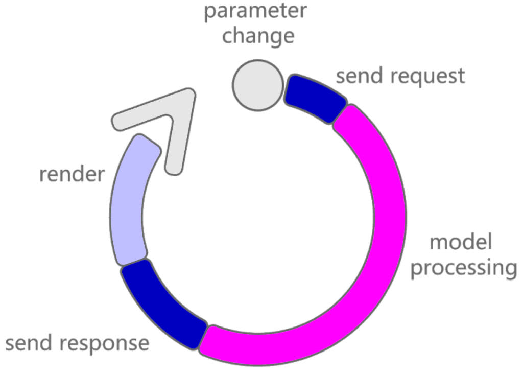
Finally, the updated model is received by our viewer and displayed (rendered) in the web browser in all its glory. The number and size of the meshes to be displayed also influences the time it takes the viewer to parse and display the geometry. It is also a good practice to hide all geometry that does not need to be displayed. As an example, nested curves for manufacturing do not need to be shown. If you have a dedicated graphics card, assign it to the browser in card settings for a better experience.

Learn more about meshing in this webinar.

Advanced Cases

It is not uncommon to hit computation time limits even with thorough optimisation, especially when the model contains logic for exporting manufacturing data. This obstacle can be overcome by controlling the Grasshopper definition and triggering output processes on demand with a toggle. Outputs used for manufacturing do not need to be computed every time a parameter changes but only at the very end of the configuration process.

In the most advanced setups, it is even possible to use the backend API to request computationally intense operations asynchronously and separate this step from the interaction phase completely.

Read more about our backend API.

Bottom Line

Cloud applications can be a powerful tool, though there's certainly a learning curve when coming from a "non-cloud" background. With a combination of documentation, video tutorials, and free support, we're aiming to give our users all the right tools needed to get started building their very own online tools!

<< If you have any questions, make sure to let us know via our Forum. Our development team is ready to assist you free assistance and troubleshooting! If you need to upgrade your account and increase your computation time, head to our website and reach out to us via our contact form. >>